Airglow Problems in High Source Density Scans
Overview
In anticipation of the last leg of observations we have looked over a population
of high source density scans and identified ~70 that may be suffering from
airglow problems and should possibly be reobserved as the opportunity exists
between gathering the final scans in the survey.
Background
Under current grading rules, airglow problems are identified by applying
a threshold to the H-band residual coadd noise (Hcn4) diagnostic. This
is very effective at identifying scans with airglow-induced ripples in
the backgrounds that will cause bad extended source problems (false sources
and bad photometry).
However, the reliability of this diagnostic breaks down in fields with
high source densities since confusion can make the background difficult
to model. We have not applied this Hcn4 diagnostic to fields with source
densities in excess of 4.2 (log of Ks souce counts per sq. degree)
because of this confusion problem, since high Hcn4 values can just as easily
crop up in scans with no airglow problems.
In Fig. 1 below, the scans currently falling within our airglow checks
are black (no airglow) and red (downgraded for airglow). The blue &
magenta point indicate scans at densities higher than those actively downgraded
for airglow.
Fig 1. Hcn(4) vs. source density diagnostic. Automatic airglow downgrades
are only applied for densities < 4.2 since the coadd noise estimates
begin to break down after this. At densities > 4.7 the Hcn(4) diagnostic
blows up as the coadd noise estimates become completely dominated by source
confusion.
Identifying Airglow in High Density Scans
In an effort to identify tiles with high densities that may also be suffering
from airglow (a condition that has not been systematically attacked before
now), I have examined the frame median background (bkg) plots for all 222
scans with source densities in the range log(Kden) = 4.2-4.7 and for which
the Hcn4 value exceeds 4.5 (these scans are plotted in magenta in Fig.
1). The bkg plots are a powerful, if qualitative, indicator of airglow
conditions since they are scaled to fit the proportions of airglow variations
(i.e. airglow variations in each band will be in similar proportions).
As a result we have produced a list of ~70 scans which have likely airglow
problems. They comprise only about 30% of the total number of scans inspected.
Of these, about half have unquestionably bad airglow variations based soley
on the erratic bkg plots. The other half are marginal but quite possibly
bad. Representative bkg plots follow:
Fig. 2: Two sample "bad" aiglow bkg plots
Fig. 3: Two plots with "marginal" airglow bkg plots
Following are two sets of coadd images for scans picked arbitrarily
from the list of bad and marginal tiles. Both show obvious airglow.
While only 3 coadds are displayed in this quick priview,
T. Jarrett has inspected both scans in their entirety and found significant
airglow throughout.
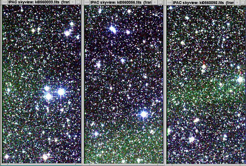
Fig. 4a: "Moderate" airglow scan 990610s 056
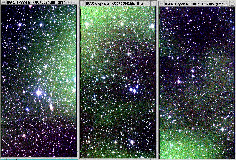
Fig 4b: "Bad" airglow scan 990726s 007
We have also inspected 3 scans from 980624s including 2 "moderate" (110-111) and
1 "bad" (112) scans. All show airglow effects throughout, with the "bad" field
consistently worse with sharp changes in background. The severity of airglow
in all of the inspected scans correlates well with the new diagnostic discussed
below.
List of suspect tiles
The first table is of the definitely bad tiles, while the second contains
the sample with marginal background plots. It is possible to further reduce
this list by inspecting coadds taken off of the image server but we have
not attempted this yet.
Bad airglow tiles
Tile DateHemi Scan Kdens Hcn4
311055    980624s    112      4.25    11.1
324473    990620s    016      4.27    17.4
324475    990620s    018      4.32     4.7
322965    990626s    037      4.51    11.9
322966    990626s    038       4.5     8.7
322967    990626s    039      4.48     5.5
322985    990626s    069      4.31     6.2
322987    990626s    071       4.3      13
322988    990626s    072      4.28     5.7
322989    990626s    079      4.28     7.4
322990    990626s    080       4.3     9.3
322997    990626s    093      4.21     5.7
323022    990724s    050      4.23     5.7
205399    990724s    094      4.28    12.3
324444    990725s    020      4.26     4.6
324415    990726s    007      4.28       6
324416    990726s    008       4.3    16.1
324417    990726s    009      4.28      11
324418    990726s    010      4.29    12.1
324442    990726s    013      4.27     6.1
324446    990726s    014      4.26    12.1
324467    990726s    021       4.3    13.5
324478    990726s    022      4.29     9.7
202412    990801s    089      4.24     6.5
202413    990801s    090      4.23    10.6
202330    990807s    075      4.57    10.3
305308    990820s    014      4.67    42.3
21266     991121n    012      4.29     7.3
324381    000126s    103      4.35     5.2
11160     000422n    092      4.61      11
326065    000423s    028      4.63    20.2
322990    000611s    047      4.26       9
322991    000611s    048      4.27       6
302368    000611s    074      4.64     7.2
322990    000717s    021      4.29     4.9
Marginal airglow tiles
Tile      DateHemi   Scan    Kdens    Hcn4
11110     970614n    098      4.28     5.3
11112     970614n    100      4.32     7.7
11167     970617n    072      4.59     9.9
11168     970617n    073      4.57      11
11187     970617n    104      4.35     5.7
308234    980416s    121      4.22     6.3
16496     980430n    085      4.33     7.3
311053    980624s    110      4.31       8
311054    980624s    111      4.28     7.3
305217    990426s    089       4.4     5.3
320840    990610s    056      4.53     5.9
320842    990610s    058      4.56     5.2
320844    990610s    060      4.59     5.9
320846    990610s    061      4.59       5
324495    990620s    051      4.32     6.7
324497    990620s    053      4.31     4.9
322976    990626s    054      4.41     5.2
322978    990626s    056      4.35     4.8
322979    990626s    057      4.38     6.8
322982    990626s    066      4.35    12.7
322983    990626s    067      4.34     5.2
322984    990626s    068      4.34       5
322986    990626s    070      4.31     4.8
322991    990626s    081      4.25     5.1
322992    990626s    082      4.24     6.2
322994    990626s    084      4.23     4.7
320962    990715s    086       4.5     5.6
205396    990721s    101       4.3    11.9
205397    990721s    102      4.28     8.4
205398    990721s    103       4.3    11.8
202409    990801s    086      4.32     4.6
205363    990804s    073      4.68    17.6
205366    990804s    076      4.62    14.7
202326    990807s    071      4.54     5.8
202328    990807s    073      4.54     9.6
202332    990807s    077      4.61     5.6
21295     991022n    017      4.27     5.6
21267     991121n    013      4.27     7.3
21268     991121n    014      4.29     7.9
21273     991121n    022      4.29     7.2
21275     991121n    024      4.27     7.5
326142    000502s    041      4.67     4.8
302367    000611s    073      4.65    18.5
Other Diagnostics
In looking over the scan characteristics of this set of visually-selected
problem tiles, there is one kind of diagnostic that correlates extremely
well with the tiles found to have airglow problems. This potential new
diagnostic is derived from the coadd banding diagnostic counters. These
tally the number of coadds in a scan found to have banding in excess of
a 5-sigma threshold based on Fourier analysis of the right and left sides
of the coadds. This was originally devised to catch J electronics banding
found early in the project, but the diagnostic also correlates well with
airglow.
In order to isolate H-band airglow problems using the Airglow Banding
Diagnostic (ABD) values, we construct a new indicator of the form:
airglow banding diagnostic = 2(Hbl + Hbr) - (Jbl + Jbr + Kbl
+ Kbr)
where the term represent the "l"eft and "r"ight banding counts for each
band. Each term can be in the range of 0-23. Banding found evenly
across all bands (i.e. not likely related to airglow) will have ABD = 0.
By subtracting the J & K banding contributions from the H contributions,
only H-strong banding seen in both halves will create large values.
The correlation between high ABD values and scans inspected for airglow
problems can be seen in the following histogram:
Fig. 5: Airglow banding diagnostic values for 3 populations of high
density scans. Red bins are for scans with confirmed bad airglow, yellow
bins show marginal evidence for airglow, and green bins are for scans clearly
not suffering from airglow. The distribution exhibits consistency between
the diagnostic and the visually-selected airglow sample.
This diagnostic is offered as food for thought on another possible
way to identify airglow problems. No statistics have yet been accumulated
for low density scans.
page last updated 9/6/00 by R. Hurt